| Modulation | QPSK (16-QAM mapper/demapper implemented, unit-verified) |
|---|---|
| FFT Size | 64 subcarriers — 48 data, 4 pilot, 1 DC null, 11 guard |
| BER at 14 dB SNR | 0 errors / 38,400 bits |
| BER at 0 dB SNR | 2.19×10⁻¹ (8,401 / 38,400 bits) |
| Frame Sync | Zadoff-Chu preamble (N=63, r=25), ~18 dB processing gain |
| Channel Model | AWGN + multipath (simulated) |
Before OFDM ever touches RF hardware, it has to work as pure math: bits in, a recognizable bit-error-rate curve out, matching what the textbook says a QPSK link should do at a given SNR. This project is that first stage — a complete OFDM physical layer written in Python, covering the same framing and synchronization structure that 802.11a, LTE, and 5G NR all use, validated against theoretical BER curves before any of it goes near a radio.
It’s explicitly scoped as Phase 1 of a larger plan. I was picking this up as a pre-research skill builder ahead of optical satellite communication work — the synchronization, channel estimation, and noise analysis techniques here carry over directly to free-space optical link acquisition and performance evaluation, just with a different physical channel underneath. Phases 2 (over-the-air on real PlutoSDR hardware via GNU Radio) and 3 (FPGA-accelerated DSP) are planned but not started — no RF hardware or RTL exists yet, and this project only claims what’s actually implemented: the software simulation.
Architecture
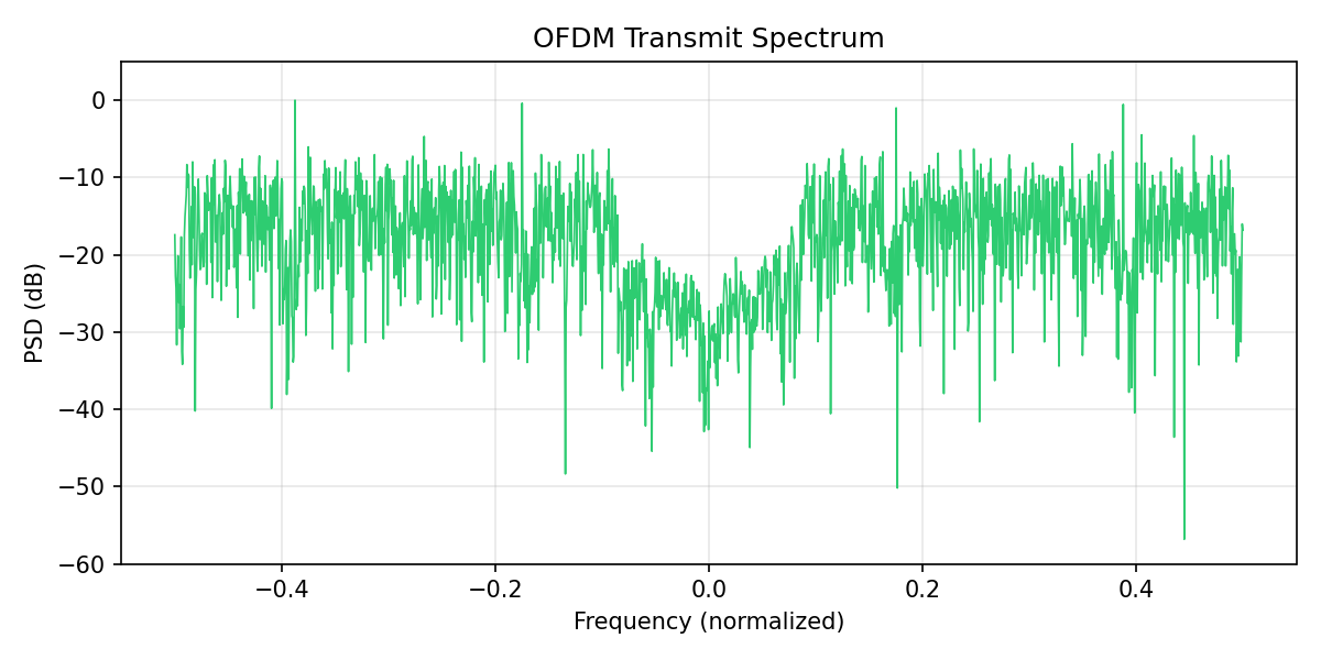
The subcarrier map follows 802.11a’s layout on a 64-point FFT:
| Subcarriers | Count | Role |
|---|---|---|
| Data | 48 | User bits, QPSK or 16-QAM |
| Pilot | 4 | Bins 11, 25, 39, 53 — known symbols for channel estimation |
| DC null | 1 | Bin 32, always zero — avoids direct-conversion DC offset |
| Guard band | 11 | Bins 0–5 and 59–63 — prevents spectral leakage into adjacent channels |
Cyclic Prefix
Each OFDM symbol gets its last 16 samples (25% of the FFT size) copied to the front before transmission:
# TX: prepend last n_cp samples
ofdm_symbol = np.concatenate([time_samples[-n_cp:], time_samples])

# RX: discard first n_cp samples
ofdm_no_cp = ofdm_with_cp[n_cp:]
That turns the channel’s linear convolution into a circular one — when a delayed multipath copy reaches back into the CP region, it finds samples identical to the symbol’s own tail, as if the signal wrapped around. After the CP is stripped at the receiver, the frequency-domain relationship is just pointwise multiplication, Y[k] = X[k] · H[k], which is what makes single-tap-per-subcarrier equalization possible at all.
Frame Synchronization
Each frame is preceded by a Zadoff-Chu sequence, the same family of sequence LTE and 5G NR use for their Primary Synchronization Signal:
It’s constant-amplitude (no clipping risk, favorable PAPR) and its periodic autocorrelation is an ideal impulse — zero at every non-zero lag — which is what makes it reliable for frame detection: the receiver cross-correlates the incoming signal against the known sequence, and the correlation peak marks exactly where the frame starts. Cross-correlation gain works out to 10·log₁₀(63) ≈ 18 dB, enough headroom to find the peak even at negative SNR.
Channel Estimation
The four pilot subcarriers are known values (1+0j) placed at fixed bins. The receiver computes a least-squares channel estimate at each pilot (H = Y/X), then linearly interpolates magnitude and phase separately across the data subcarriers between them:
for a data subcarrier at bin 18 sitting between pilots at bins 11 and 25 — closer pilots contribute proportionally more.
Verification
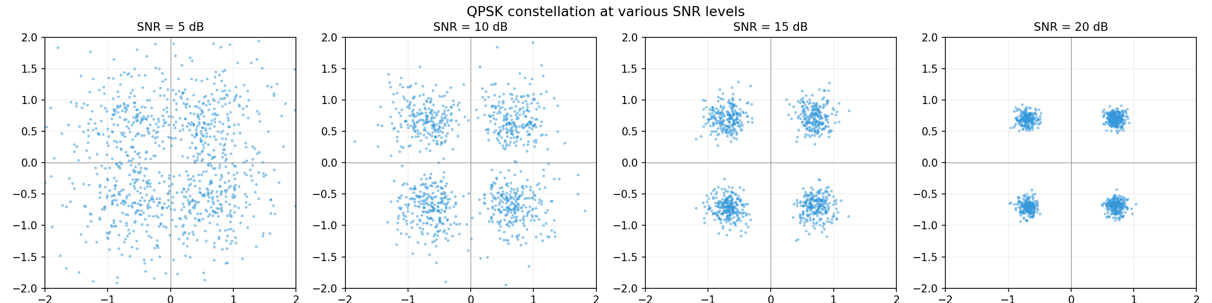
| SNR (dB) | BER (measured) | Errors / Total |
|---|---|---|
| 0 | 2.19×10⁻¹ | 8,401 / 38,400 |
| 4 | 9.20×10⁻² | 3,534 / 38,400 |
| 8 | 1.40×10⁻² | 538 / 38,400 |
| 10 | 2.89×10⁻³ | 111 / 38,400 |
| 12 | 1.56×10⁻⁴ | 6 / 38,400 |
| 14+ | 0 | 0 / 38,400 |
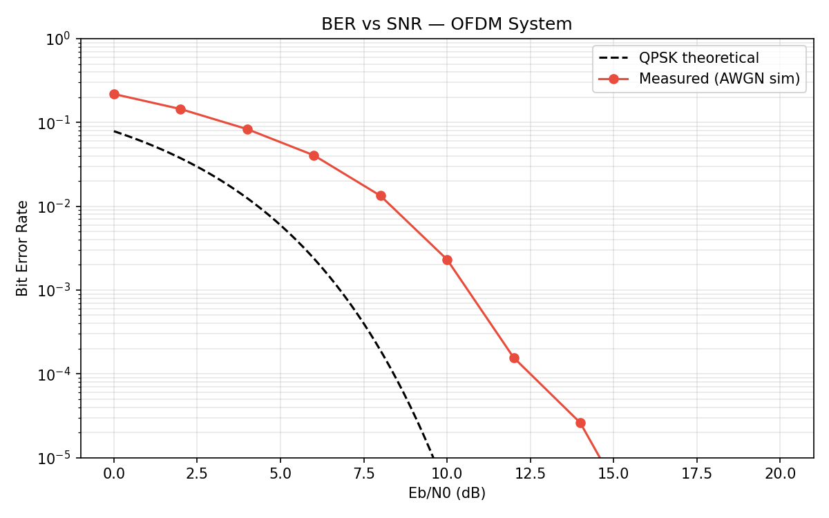
That ~2 dB gap is a real, explainable measurement result, not noise in the methodology — it’s small enough to trust the receiver chain and large enough to be worth stating honestly rather than rounding away.
The bug that got me here
The first version of this simulation didn’t produce the curve above. It produced a flat line at BER ≈ 0.483 regardless of SNR — the textbook symptom of a receiver that’s effectively guessing:
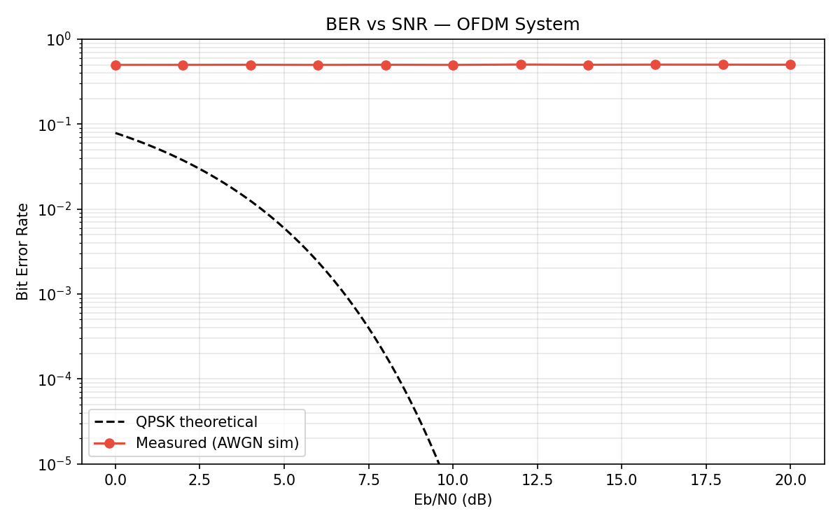
The cause was a one-character-class error in the AWGN model. Noise amplitude should scale with the square root of noise power, not noise power directly:
# Wrong: noise scales quadratically with power, not as a standard deviation
sigma = noise_power / 2

# Right
sigma = np.sqrt(noise_power / 2)
Skipping the square root meant the injected noise was enormous at every SNR setting the sweep asked for, so every symbol landed in the wrong quadrant regardless of the nominal SNR — hence a flat BER curve instead of a waterfall. It’s a one-line fix, but the debugging path to it (checking the mapper/demapper convention first, then the channel model) is the more useful part: a flat, SNR-independent BER points at something structurally broken in the link, not a subtle tuning issue, and it’s worth ruling out the “big” bugs before chasing precision losses.
Up Next
Phase 1 — the software simulation on this page — is complete and verified. Phase 2 (real over-the-air transmission between two ADALM-PlutoSDR boards via GNU Radio) and Phase 3 (FPGA-accelerated FFT and correlator) are the planned next steps, not yet started. Nothing on this page claims real RF hardware or FPGA acceleration until that work actually exists.